Fundamentals of Radiance Cascades

Introduction

In this article I'm going to share my understanding of the fudamentals of Radiance Cascades. (abbreviated as RC)
Over the past months I've build some intuitions & understanding of RC, and my goal is to share some of that here with you.

This article will likely be easier to follow for those with prior experience with ray tracing & global illumination.
Nevertheless, I'll do my best to explains everything in an intuitive way using graphics!

At it's core, Radiance Cascades is a method for efficiently representing a radiance field (light field).
Which allows us to represent the incoming light from/around some area at any point within that area.
In 2D that area is usually the screen.

For the sake of simplicity I will explain everything in 2D, however RC can be expanded into 3D aswell.

So, what can RC in 2D (also referred to as Flatland) achieve?
My implementation is able to compute diffuse global illumination in real-time:

An awesome property of this method is that this is done fully-deterministically!
Furthermore, there are already plenty of clever ways to get its performance to acceptable levels for modern hardware.

So without further ado, let's dive in!

Observations

Radiance Cascades is built on two key observations.
So first, let's observe these together, and have a short recap afterwards.

But, before we observe anything I want clear up what I mean with the following terms:

1. radiance: light from a specific direction, at a specific point. (You can think of this as a ray)
2. irradiance: light from a subset of directions, at a specific point. (You can think of this as light from all directions)

Because radiance is just one direction, we can build irradiance from a bunch of directions (radiance).

Angular Observation

Figure A, depicts a circular object on the left, with a radiance probe to the right of it.
The radiance probe has an angular resolution which can be defined as the angle between its evenly spaced rays. (Shown in blue)
As the radiance probe moves further away from the light source, we can see that its angular resolution becomes insufficient.

What we can observe here is that the angle between rays we can get away with for a probe, depends on two factors:

1. $ D $ The distance to the furthest object.
2. $ w $ The size of the smallest object.

In the paper this restriction is formalized with this equation: $ \Delta_\omega < w/D $
Which states that the angle between our evenly spaced rays $ \Delta_\omega $ should be smaller than $ w/D $.

Spatial Observation

Figure B, shows that we can resolve a penumbra by interpolating between only 2 probes. (Shown as blue dots)
The spacing of these probes can be increased the further away we get from all objects in the scene.

We can observe that the probe spacing is dependent on two factors:

1. $ D $ The distance to the closest object.
2. $ w $ The size of the smallest object.

Does that not sound familiar?

The distance is the inverse of the angular observation!

Figure C, shows that regardless of the distance between the light and the occluder, the penumbra still grows with distance.
However, the sharpness of the penumbra changes, RC is notoriously bad at representing very sharp shadows.

Figure C, also serves to highlight that we're interested in the nearest or furthest object, not light source.
At the end of the day, a wall is just a light source that emits no light, and a light source is just a wall that emits light.

Penumbra Condition / Theorem

While the required angle between rays ($ \Delta_\omega $) decreases, the required distance between probes ($ \Delta_p $) increases and vice versa.
They are inversely proportional.

In the paper this relationship is formalized as the penumbra condition with this equation:

$ \begin{cases} \Delta_p <\sim D, \\ \Delta_\omega <\sim 1/D \end{cases} $

$ A <\sim B $ means that; $ A $ is less than the output of some function, which scales linearly with $ B $.

$ w $ (the size of the smallest object) is not included in the penumbra condition because it is the same at all points in the scene.
We can also observe that the required angular & spatial resolution both increase when $ w $ decreases.
Because we need higher resolution for both in order to resolve the smallest object in the scene.

Recap

Ok, these observations took me some time to wrap my head around but they're key to understanding RC.
So let's quickly reiterate our observations.

What we've observed is that the further we are from the closest object in the scene:

1. The less spatial resolution we need. (e.g. the larger spacing can be between probes)
2. The more angular resolution we need. (e.g. the more rays we need per probe)

Exploiting Observations

Now that we've made the observations and defined the penumbra theorem, let's look at how we can exploit these observations.

Angular

We've got a problem: classic probes we're all used to, can hit objects at virtually any distance.
In order to exploit the penumbra theorem we need some way to narrow this possible distance window.

Figure D, shows one way of narrowing this window, we can discretize our circular probes into rings.
By doing this we not only know that each ring will hit within a narrow distance window,
we can also vary the angular resolution between rings!

These new rays with a limited range, are referred to as intervals.

This is exactly what we're looking for to exploit the angular part of the penumbra theorem.
We can increase the interval count (aka, decrease the angle between rays) with each consecutive ring that hits objects further away.

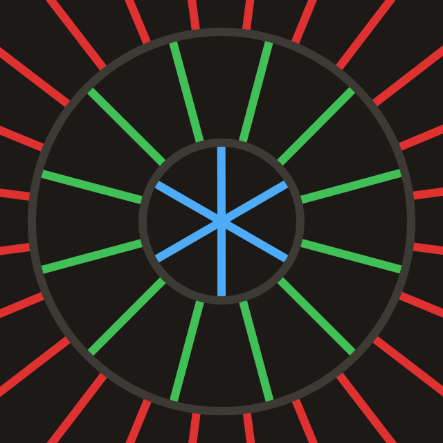Figure E: Increasing angular resolution for more distant “rings”.

In order to still capture our entire scene, we will have many of these rings.

In the example in Figure E, we increase the interval count by 2x with every consecutive ring.
Which let's us increase the distance window of each ring (the length of its intervals) by that same factor.
This ensures the gap between intervals remains approximately equal between rings.

Spatial

So far, with the angular observation we haven't really achieved any reduction in ray count.
We're still casting a very large number of rays for each probe using this method, good thing that's about to change.

This is when we drop the idea that these rings together make up a single probe.
Instead, let's view each consecutive ring as its own probe, which can be moved.

From now on when we refer to probes, we are referring to rings.

The length of the intervals in Figure F is incorrect, this is to make them easier on the eyes.

Figure F, shows one way we can use this new perspective on the probes.
We saw during the spatial observation that when objects are further away, we can have larger spacing between probes.

So, when our distance window gets further and further away, we may increase the spacing between those probes.
And because we're trying to fill some area with them, this means we need less of them.

There is a visible disconnect between probes between cascades, this does result in artifacts, mainly ringing.

There are fixes out there (e.g. bilinear & parallax fix), however they're out of the scope of this article.

Cascades

Now that we understand how we can exploit the two key observations.
Let's put the two together and finally define what exactly a cascade is!

Figure G1: Cascade 0, with 4x4 probes.

Figure G2: Cascade 1, with 2x2 probes.

A cascade is basically a grid of probes, in which all probes have equal properties.
(e.g. interval count, interval length, probe spacing)

The reason we call them cascades is because they cascade outwards with increasing interval count and length.
Or at least, that's how I like to think about it.

Cascade Hierarchy

A cascade on its own isn't super useful, only capturing a small part of the scene.
Many cascades together is what we're really after, we want to combine them into a hierarchy.
For example in Figure G1 & G2 we can see two cascades that could make up a cascade hierarchy.

Most of the time, for simplicity sake we will decrease probe count between cascades by 2x along each axis.
Like we've seen also in Figure G1 & G2, we will find out why this is convenient later on in this article.

If we're following the penumbra condition, the spatial and angular resolution should be inversely proportional.
So if we increase probe spacing by 2x we need to decrease the angle between intervals by 2x as well.

However, there's also many implementation which decrease the angle between intervals by 4x instead.
It is more costly, but it may produce higher quality results in some cases.

Cascade Memory

The most common way we store probes in memory is using a 2D texture.
In Figure H, we can see one such probe, it has 16 intervals making it 4x4 texels in memory.
Each texel representing a single direction, indicated by the white arrow in the center.

const int dir_count = 16; /* 4x4 */
const int dir_index = ...;

/* Compute interval direction from direction index */
float angle = 2.0 * PI * ((float(dir_index) + 0.5) / float(dir_count));
vec2 dir    = vec2(cos(angle), sin(angle));

The code snippet above shows how we can derive an interval direction from its index within its probe.

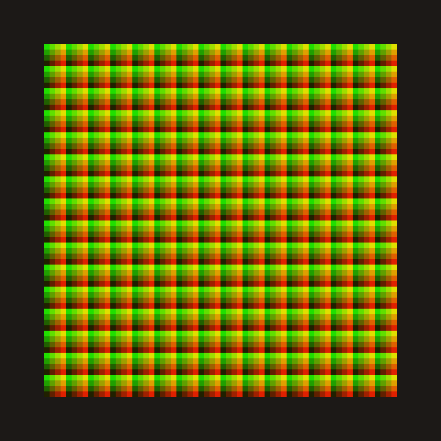Figure I: Cascade in texture memory.

Now, of course we're not going to store each probe in its own texture.
Instead, let's store each cascade in a texture, packing the probes together as shown in Figure I.

There's also an alternative superior data layout, called direction first.
Where you store all intervals with the same direction together in blocks, which improves data locality during merging.

This is where we see why decreasing the probe count by 2x on each axis is nice.
It works out really well when using this kind of packing.

If we decrease the angle between intervals by 2x each cascade, each subsequent cascade will have half the intervals of the previous.
Because the probe count is decreasing by 2x along 2 axes, making it decrease by 4x, while the interval count only increases by 2x.

Meaning our total interval count will aproach 2x the interval count of the first cascade as we add more cascades.

If instead, we decrease the angle between intervals by 4x each cascade, each cascade will have equal the intervals.

Meaning our total interval count will grow linearly with cascade count.

I recommend using the 4x branching method where interval count remains equal, it is simpler to work with in practice.

Cascade Gathering

To gather the radiance for each cascade we simply loop over each texel in its memory texture.
For each of those texels we calculate the direction and cast our interval into the scene.

First, let's find out what our coordinate is within the probe we're apart of:

/* Get the local texel coordinate in the local probe */
const ivec2 dir_coord = texel_coord % probe_size;

Second, we can convert this coordinate to a direction index:

/* Convert our local texel coordinate to a direction index */
const int dir_index = dir_coord.x + dir_coord.y * probe_size.x;

Third, using that direction index we can obtain the direction vector: (like I showed earlier)

const int dir_count = probe_size.x * probe_size.y;

/* Compute interval direction from direction index */
float angle = 2.0 * PI * ((float(dir_index) + 0.5) / float(dir_count));
vec2 dir    = vec2(cos(angle), sin(angle));

Now we have to cast the interval, let's not forget intervals have a start and end time:

vec2 interval_start = probe_pos + dir * start_time;
vec2 interval_end   = probe_pos + dir * end_time;
vec3 radiance       = cast_interval(interval_start, interval_end);

It's important to note, the cast_interval function can use whatever ray casting method you want.
As long as it returns the radiance information from the scene from the start to the end position.

The start & end time of our intervals depends on which cascade we're evaluating, and what branching is used.
For 4x branching (the branching I recommend) we can use this code to find the start & end times:

/* Get the scale factor for an interval in a given cascade */
float interval_scale(int cascade_index) {
    if (cascade_index <= 0) return 0.0;

    /* Scale interval by 4x each cascade */
    return float(1 << (2 * cascade_index));
}

/* Get the start & end time of an interval for a given cascade */
vec2 interval_range(int cascade_index, float base_length) {
    return base_length * vec2(interval_scale(cascade_index), interval_scale(cascade_index + 1));
}

The base_length above is the length you want intervals in cascade0 to have.

Merging

Now we have our radiance field stored as cascades in textures. Awesome!
The next step is to extract the data we want from this data structure (the cascade hierarchy).

We're going to extract specifically the diffuse irradiance of the scene. (also called fluence in 2D)
This basically means summing up the radiance coming from all directions for a specific point.

Merging Intervals

We've talked about basically splitting our rays into seperate intervals, probes => rings.
So how can we connect those seperate intervals back again, to make up a ray?

In Figure J, we can see that intervals earlier in the chain can occlude intervals further down the chain.
To properly resolve this relation, we usually use a ray visibility term which is stored in the alpha channel.
This term is set during the initial gathering, it is 1.0 if the interval hit nothing, and 0.0 if it did.

/* Merge 2 connected intervals with respect to their visibility term */
vec4 merge_intervals(vec4 near, vec4 far) {
    /* Far radiance can get occluded by near visibility term */
    const vec3 radiance = near.rgb + (far.rgb * near.a);

    return vec4(radiance, near.a * far.a);
}

The code snippet above shows how we can implement interval merging in code.
As we can see, radiance from the far interval can be occluded by the visibility term of the near interval.

We also merge the visibility terms, by multiplying them a hit will also be carried downwards. (1.0 * 0.0 = 0.0)

Merging Cones

It would be really expensive if we had to merge through each cascade for each possible direction.
So instead, let's merge each cascade into the one below it, from the top down.

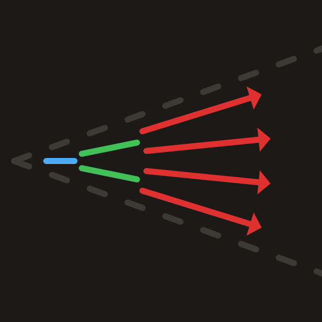Figure K: Cone made out of intervals.

Because we're trying to extract diffuse lighting, directional resolution isn't very important.
So it's completely fine to squash the entire scene radiance into cascade0 (which has the lowest angular resolution)

Because we have a branch factor, e.g. 4x, each cascade we will merge 4 intervals down into 1 interval.
Doing so for all cascades recursively captures the radiance from a cone, as shown in Figure K.

This is perfect for capturing our low angular resolution diffuse lighting!

Merging Spatially

Not only our angular resolution changes between cascades, we also know our spatial resolution changes.
If we always merge with the nearest probe from the next cascade, we will get an obvious grid pattern.

The "next cascade" is the cascade above the current one, it has lower spatial & higher angular resolution.

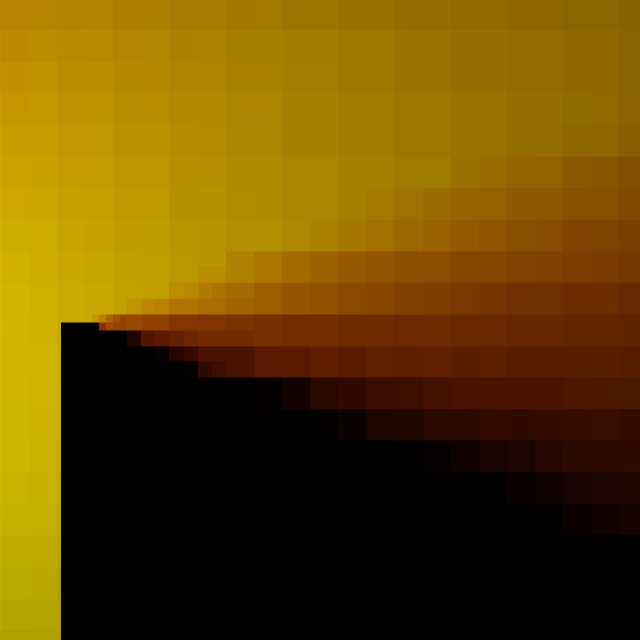Figure L: Merging with nearest probe only.

In Figure L, we can clearly see this obvious grid pattern, which actually visualizes the probes themselves.
It is a cool effect, but not exactly the smooth penumbrae we're looking for.

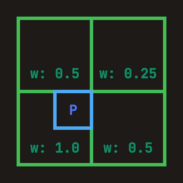Figure M: Merging with 4 bilinear probes.

Weights shown in Figure M are incorrect! They should always add up to 1.0.

Let's instead use bilinear interpolation to merge with the nearest 4 probes from the next cascade.
We can see what this looks like in Figure M, bilinear probes closer to the destination probe get higher weights.

I like to think of it as blurring those blocky probes in Figure L with their neighbours.

I tend to refer to the green probes as "bilinear probes" & the blue probe as "destination probe".

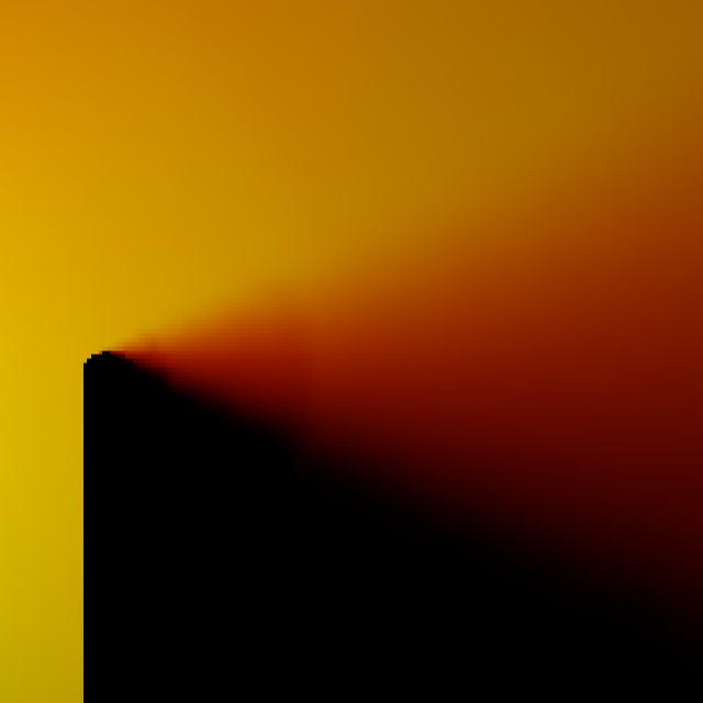Figure N: Smooth penumbrae using bilinear interpolation.

In Figure N, we can see the effect of spatially interpolating the probes using bilinear interpolation.
The result is nice smooth penumbrae, instead of the blocky ones we got with nearest interpolation.

Merging Algorithm

Let's put our angular & spatial merging together to finally obtain our diffuse lighting.

Remember, we merge top down, starting with the lowest spatial resolution going down to the highest spatial resolution.

Starting from the top, the first cascade doesn't have a cascade to merge with.
We can either skip it, or we can merge with a skybox for example.

For every other cascade we will merge with the one above it, we can write this as: $ N_{i+1} \to N_{i} $
From now on I'll be referring to them as N+1 and N for simplicity.

The first step is finding our 4 bilinear probes from N+1, and their respective weights.
To find the 4 bilinear probes we get the top-left bilinear probe index, and then simply iterate over a 2x2 from that base_index.
And we'll use the fractional part of that base_index to derive our bilinear weights:

/* Sub-texel offset to bilinear interpolation weights */
vec4 bilinear_weights(vec2 ratio) {
    return vec4(
        (1.0 - ratio.x) * (1.0 - ratio.y),
        ratio.x * (1.0 - ratio.y),
        (1.0 - ratio.x) * ratio.y,
        ratio.x * ratio.y
    );
}

void bilinear_samples(vec2 dest_center, vec2 bilinear_size, out vec4 weights, out ivec2 base_index) {
    /* Coordinate of the top-left bilinear probe when floored */
    const vec2 base_coord = (dest_center / bilinear_size) - vec2(0.5, 0.5);

    const vec2 ratio = fract(base_coord);  /* Sub-bilinear probe position */
    weights = bilinear_weights(ratio);
    base_index = ivec2(floor(base_coord)); /* Top-left bilinear probe coordinate */
}

As inputs our bilinear_samples takes the following parameters:

vec2 dest_center = ...; /* Center position of destination probe in pixels */
vec2 bilinear_size = ...; /* Size of bilinear probe in pixels */

Now we will have 2 nested loops:
For each of the 4 bilinear probes, we will merge with 4 of their intervals.

/* For each extra N+1 interval */
for (int d = 0; d < 4; d++) {
    /* For each N+1 bilinear probe */
    for (int b = 0; b < 4; b++) {
        const ivec2 base_offset = bilinear_offset(b);

        /* ... */
    }
}

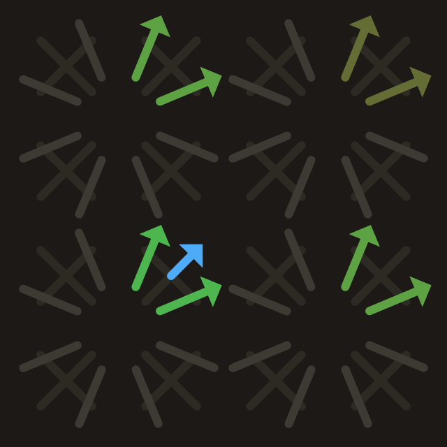Figure O: Merging for 1 interval (in blue).

Looking at Figure O, we get a visual of what those nested loops are for.
Looping over the 4 nearest probes from N+1 and (in this graphic 2) intervals.
Figure O is drawn with a branch factor of 2x instead of our 4x otherwise it can get quite busy with all the intervals.

The green intervals in Figure O are colored based on their bilinear weights, brighter means a higher weight.

You may have noticed the bilinear_offset function in the inner loop.
It simply converts our 1D index into a coordinate in the 2x2 bilinear square:

/* Convert index 0..4 to a 2d index in a 2x2 square */
ivec2 bilinear_offset(int offset_index) {
    const ivec2 offsets[4] = { ivec2(0, 0), ivec2(1, 0), ivec2(0, 1), ivec2(1, 1) };
    return offsets[offset_index];
}

We can add our base_offset to the base_index we got earlier to get the 2D index of the bilinear probe.

/* Get the index of the bilinear probe to merge with */
const ivec2 bilinear_index = base_index + base_offset;

Now it is relatively trivial to use our dir_index we learned how to get earlier.
To get a directional base_index and add d to it.

/* Get the directional base index */
const int base_dir_index = dir_index * 4;

/* Get the directional index we want to merge with */
const int bilinear_dir_index = base_dir_index + d;

Then finally we can combine the bilinear_dir_index & bilinear_index to get the texel coordinate in cascade N+1 to merge with.

/* Convert the directional index to a local texel coordinate */
const ivec2 bilinear_dir_coord = ivec2(
    bilinear_dir_index % bilinear_size.x,
    bilinear_dir_index / bilinear_size.y
);

/* Get the texel coordinate to merge with in cascade N+1 */
const ivec2 bilinear_texel = bilinear_index * bilinear_size + bilinear_dir_coord;

Merging we do using the merge_intervals function from earlier in the article.

/* For each extra N+1 interval */
vec4 merged = vec4(0.0);
for (int d = 0; d < 4; d++) {
    /* For each N+1 bilinear probe */
    vec4 radiance = vec4(0.0);
    for (int b = 0; b < 4; b++) {
        /* ... */

        /* Fetch the bilinear interval from the cascade N+1 texture */
        const vec4 bilinear_interval = textureFetch(bilinear_texel);

        /* Merge our destination interval with the bilinear interval */
        radiance += merge_intervals(destination_interval, bilinear_interval) * weights[b];
    }

    merged += radiance / 4.0;
}

That's all! We've now merged all the cascades down into cascade0.

Final Pass

I did say "that's all", I know, I know, but there's one more step,
which is to integrate the irradiance stored in the now merged cascade0.

Luckily this is relatively trivial, we already have most of the code we need.
We simply bilinearly interpolate between the 4 nearest cascade0 probes for each pixel.
And sum up the radiance from all intervals. (cones)

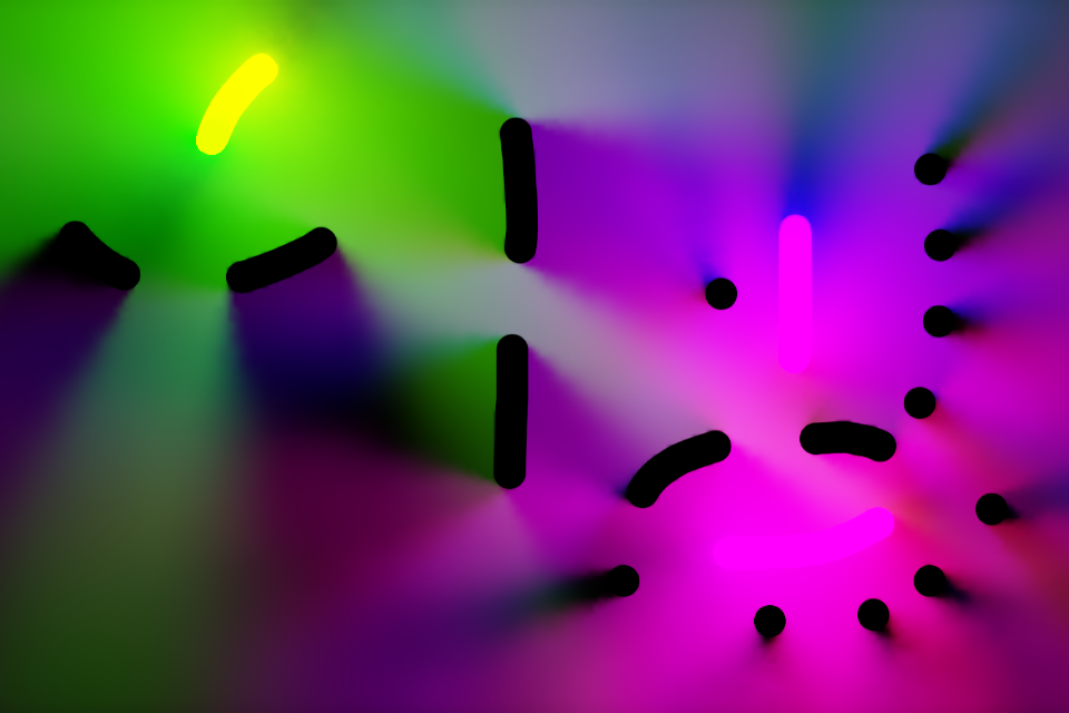Figure P: Final result! (Credit: Fad's Shadertoy)

Image credit: Fad's Shadertoy.

If we did everything correctly, we should end up with a beautiful result like in Figure P.

For those who made it all the way till the end, thank you for reading my article!
I hope it sheds some light on how & why Radiance Cascades work.
It took me a while to properly understand it, and a lot of trial & error to get it working :)

Amazing Resources

There's quite a few resources already out there related to RC. (which also helped me)
I will list a few of them here, so you can get explanations from different perspectives:

• Alexander Sannikov's paper on Radiance Cascades.
• XorDev & Yaazarai's articles, part 1 & part 2.
• SimonDev's video https://youtu.be/3so7xdZHKxw.
• Christopher M. J. Osborne's paper diving deeper into the bilinear fix.
• Jason's blog post https://jason.today/rc.
• Fad's Shadertoy implementation.

Also check out our Discord community there's a lot of awesome people there that might be able to help you out!